Fortunately, if a condition of vocabulary balance does exist in a given sample of speech, we shall have little difficulty in detecting it because of the very nature and direction of the two Forces involved. On the one hand, the Force of Unification will act in the direction of decreasing the number of different words to 1, while increasing the frequency of that 1 word to 100%. Conversely, the Force of Diversification will act in the opposite direction of increasing the number of different words, while decreasing their average frequency of occurrence towards 1. Therefore number and frequency will be the parameters of vocabulary balance.
Since the number of different words in a sample of speech together with their respective frequencies of occurrences can be determined empirically, it is clear that our next step is to seek relevant empiric information about the number and frequency of occurrences of words in some actual samples of speech.
(George K. Zipf, Human Behavior and the Principle of Least Effort, 1949)
segunda-feira, 13 de dezembro de 2010
Double superlatives
Yet when we offer a prize to the submarine commander who sinks the greatest number of ships in the shortest possible time, we have a double superlative -- a maximum number and a minimum time -- which renders the problem completely meaningless and indeterminate, as becomes apparent upon reflection. Double superlatives of this sort, which are by no means uncommon in present-day statements, can lead to a mental confusion with disastrous results.
As pointed out years ago, the frequent statement, "in a democracy we believe in the greatest good for the greatest number," contains a double superlative and therefore is meaningless and indeterminate. (In Part Two we shall see that the distribution of goods and services are in fact governed by a single superlative.) Intimately connected with the "singleness of the superlative" is what might be called the singleness of the objective whose implications are often overlooked (i.e., the pursuit of one objective may preclude or frustrate the pursuit of the scoond objective). These two concepts apply to all studies in ecology.
(George K. Zipf, Human Behavior and the Principle of Least Effort, 1949)
segunda-feira, 6 de dezembro de 2010
Mandelbrot Set

The Mandelbrot set M is defined by a family of complex quadratic polynomials
$P_c:\mathbb C\to\mathbb C$
given by
$P_c: z\mapsto z^2 + c$, where c is a complex parameter.
If the sequence $(0, P_c(0), P_c(P_c(0)), P_c(P_c(P_c(0))), \ldots)$ (starting with $z=0$) does not escapes to infinity, the complex number c is said to belong to the set.
A simple Octave/Matlab code was created to plot the complex numbers on the Mandelbrot set.
mset=[];
x=[-2:0.001:1];
y=[-1:0.001:1];
k=0;
for k1=1:length(x),
for k2=1:length(y),
    c=x(k1)+i*y(k2);
    z=0;
    for it=1:100,
        z = z^2+c;
    end;
    if(z < Inf), k++; mset(k)=c; end;
end;
end;
figure; plot(mset,'k.');
terça-feira, 30 de novembro de 2010
Simulation on Sand Avalanches
It is common to observe how complex systems in nature present similar patterns, what is due to the self-organized criticality. Critical points work as attractors towards which systems evolve seeking for equilibrium. A common example are the sand piles. It is observed that as more grain of sand are dropped, new avalanches may occur. The avalanches may be of different proportions, local small avalanches or big ones, spreading widely in the pile. The observation of these avalanches shows that they follow a Zipf's law.
Here I present the results of a simulation of sand avalanches. The video shows a set of samples, which with 10 continuous seconds taken every 80 seconds from the simulation. At every second a new sand is randomly dropped on the board. If a certain peak has 4 more grain of sand then any of its neighbours, an avalanche happens towards this neighbour, what might lead to a cascade of avalanches.
The histogram bellow show the frequency of occurrence of avalanches of different sizes, described as: 0 (no avalanche), 1 (avalanche happened just on the level the grain was dropped), 2 (avalanche spreads to the next level), and so forth.

If we present the result above as a log-log plot of the types of avalanches (according to their magnitude) ranked according to their frequency of occurrence, we get to the figure bellows, which clearly is a power law, a Zipf's law. The type of avalanche with rank one is the most frequent, the type ranked two is the second most frequent, and so on. The plot bellow shows the rank vs. frequency of occurrence. The numbers presented near the curve (1 2 3 0 4 5 6 ...) are the type of avalanche: 1 stands for avalanche only in the level where the grain is dropped; 2 when the avalanche spreads to the next level; 3 when it spread two levels bellow; 0 when there is no avalanche; etc.

sexta-feira, 26 de novembro de 2010
Zipf's Law
Zipf's statistical law is based on the idea that two "opposing forces" are in constant operation in a system. In the stream of speech, they are: the Force of Unification and the Force of Diversification. Any speech is is a result of the interplay of these forces, that through a self-organizing process reaches a critical point, a point of "balance" between them. This balance is observed on the relation between the frequency of occurrence of words (f) and their rank (k), their product is constant.
$f(k;s,N)=\frac{1/k^s}{\sum_{n=1}^N (1/n^s)}$.
In the formula above, s stands for the exponent that characterizes the distribution; and N stands for the number of elements in the set. The formula states that the frequency of occurrence of a given element is given by the rank of this element within a given, which distribution is characterized by s. The figure bellow presents how the relationship of frequency and rank is when plotted in a log-log scale for different values of s.

Zipf developed the idea using an intrinsic linguistic or psychological reason to explain this phenomena observed in the world of words. He named his theory the "Principle of Least Effort" to explain why frequently encountered words are chosen to be shorter in order to require a little mental and physical effort to recall them and utter/write them. According to Alexander et al. (1998), Zipf’s law seems to hold regardless the language observed. "Investigations with English, Latin, Greek, Dakota, Plains Cree, Nootka (an Eskimo language), speech of children at various ages, and some schizophrenic speech have all been seen to follow this law"(Alexander et al., 1998).
The Zipf’s law is also observed in other phenomena, for example: the magnitude of earthquakes (it is common to have many small earthquakes, but big ones are rare) (Abe and Suzuki, 2005); the population in cities (there are few megalopolis, but thousands of small cities) (Gabaix, 1999); the distribution of total liabilities1 of bankrupted firms in high debt range(Fujiwara, 2004); the number of requests for webpages(Adamic and Huberman, 2002); etc.
The observation of languages also points to a Zipf’s law, what makes one more evidence that languages operate in a rather random way. Performing a statistical analysis of language means to acknowledge its unpredictable nature, without which there would be no communication at all. The analysis of languages as a statistical process has advantages over the qualitative analysis, it "is able to afford to neglect the narrow limits of one language and concentrate on linguistic problems of a general character" (Trnka, 1950). Although this conflict between randomness and rationality might rise suspicious on the character of languages, Miller wisely pointed: "If a statistical test cannot distinguish rational from random behavior, clearly it cannot be used to prove that the behavior is rational. But, conversely, neither can it be used to prove that the behavior is random. The argument marches neither forward nor backward" (Miller, 1965).
References:
Abe, S. and Suzuki, N. (2005). Scale-free statistics of time interval between successive earthquakes. Physica A: Statistical Mechanics and its Applications, 350(2-4):588–596.
Adamic, L. A. and Huberman, B. A. (2002). Zipf’s law and the internet. Glottometrics,
3:143–150.
Alexander, L., Johnson, R., and Weiss, J. (1998). Exploring zipf’s law. Teaching Mathe
matics Applications, 17(4):155–158.
Fujiwara, Y. (2004). Zipf law in firms bankruptcy. Physica A: Statistical and Theoretical Physics, 337(1-2):219–230.
Gabaix, X. (1999). Zipf’s law for cities: An explanation. Quarterly Journal of Economics, 114(3):739–67.
Miller, G. A. and Taylor, W. G. (1948). The perception of repeated bursts of noise. The Journal of the Acoustical Society of America.
Trnka, Bohumil (1950). Review of: G.K.Zipf, The psychobiology of language. Human behavior and the principle of least effort.
sábado, 20 de novembro de 2010
The minimum wage miracle
With the new Constitution of 1988, it was granted to every worker, the right to earn at least an amount called "minimum wage". In the second chapter, sixth article, it defines this minimum wage as the amount capable of attending the basic vital necessities of a worker and his family with home, food, education, health, leisure, clothing, hygiene, transportation and social security. It is also establish, that this minimum wage should undergoes periodic readjustments to overcome inflationary degradation of the worker's purchasing power. Although the Constitution does not specifies how often those readjustments should happen and what amount should be given, we observe in the history of readjustments that there is a regularity. There is almost one readjustment every year and the readjusting factor kept following the rule: CPI (consumer price index, which is used as a measure of inflation) + percent GDP growth. The rule of readjustment followed by the government in the last years to define the readjustment factor is: the CPI of the year that has just passed plus the percent GDP growth experienced in the year before. That means: readjustment_factor[n] = CPI[n-1]*GDP[n-2]. This might be observed in the figure right bellow, where the actual minimum wage value is plotted in blue and the predicted readjustment (using the rule) in red:

It is clear now that the readjustment try to follow this rule.
The interesting point about this readjustment rule is that it promotes the distribution of wealth. As the country keeps growing, the minimum wage also keeps increasing, at a larger step. Not everyone wage keeps increasing at the minimum wage's rate. It might clearly be apprised in the figure bellow. The cyan curve shows the average wage of Brazilians. If it were to be readjusted using the same rule the minimum wage uses, it would gives us the green curve. Looking at the graphic, we see that the average wage is always bellow the green curve, what shows that, on average, the wages don't follow the minimum wage increase.

The consequence of this is better viewed when we normalized all curves by the actual minimum wage value, what is presented in the next figure.

In 1995, the average Brazilian wage was around 8 times greater than the minimum wage. In the last year, in 2009, it reached a ratio 3:1. This means distribution of wealth. Observing the curve, it seems like the curve is going to saturate at a ratio between 3:1 and 2:1, what would leave Brazil in a similar position to developed countries. Here is some ratios of average wage to minimum wage in some countries: USA 3.28:1, Spain 2.55:1, Netherlands 2.22:1, Portugal 2.02:1, France 2.00:1, UK 1.88:1 (data from: source 1 and source 2).
sexta-feira, 19 de novembro de 2010
How to deceive dumb people with exponential growth
It is pretty easy to deceive an outsider that the last few years have made a tremendous better profit in comparison to the previous ones.
When we experience a exponential growth we get surprised to see how the growth was tremendous in the last few samples. In fact, on average, the percent growth is the same, but what is important (mainly in political matters) is to convince another that we are experiencing glorious times.
A simple analysis of various examples show us percent growing rates almost constant. That is natural. Observe the GDP growth of a developing country, or the growth on the exportation, or the growth of a large company. Usually you will find a percent growing rate that is almost constant.
If we consider than a growing rate to be a random variable with a certain mean and variance, we might sketch the growing curve. Bellow I present some simulations where the percent growing rate was modeled as a normally distributed random variable with mean 4 and some distinct variances: 4, 6, 8, and 10. The growing curves are presented bellow:

And here another sketch, where the graphics are separated according to their variances.

Lets take one graphic as an example. It is plotted with its percent growth shown bellow, along with a moving average of the percent growth.

If you juts look at the first plot, you would conclude that after time 60 and/or 80 we got a bigger improvement. But you may look things in a different way. If you look at the second subplot, you may observe the percent growth through time. Now it is easy to see that it is almost the same through time, and the first picture is clearly deceiving.
Another way to see how deceiving our first graphic was is to plot the data in a logarithm scale, as shown right bellow:

Don't believe straight away on your eyes, or you might get deceived. Don't believe on exploding graphics jumping out of the paper, they are made to deceive you. Don't believe on millions and billions on a moth of a politician. To see the truth, you have to get your hands dirty.
quinta-feira, 18 de novembro de 2010
Self-Organized Criticality and Gaia
In a seminal work, Jim Lovelock, an English scientist, came up with a fascinating idea that all life on earth can be viewed as a single organism. This idea has stuck many scientists as preposterous since it flies in the face of the usual reductionist approach and smacks of New-Age philosophy. Lovelock's idea is that the environment, including the air that we breathe, should not be viewed as an external effect independent of biology, but that it is endogenous to biology. The oxygen represents one way for species to interact. Lovelock
noted that the composition of oxygen has increased dramatically since life originated. The oxygen content is far out of equilibrium. The layer of ozone, an oxygen molecule, that protects life on earth did not just happen to be there, but was formed by the oxygen created by life itself. Therefore, it does not make sense to view the environment, exemplified by the amount of oxygen, as separate from biological life. One should think of the earth as one single system.
What does it mean to say that the earth is one living organism? One might ask in general: What does it mean that anything, such as a human, is one organism? An organism maybe defined as a collection of cells or other entities that are coupled to each other so that they may exist, and cease to exist, at the same time -- that is, they share one another's fate. The definition of what represents an organism depends on the time scale that we set. ln a time scale of 100 million years, all humans represent one organism. At short time scales, an ant's nest is an organism. There is no fundamental difference between genetically identical ants carrying material back and forth to build and operate their nest, and genetically identical human cells organizing themselves in structures and sending blood around in the system to build and operate a human body.
Thus a single organism is a structure in which the various parts are interconnected, or "functionally integrated" so that the failure of one part may cause the rest of the structure to die, too. The sand pile is an organism because sand grains toppling anywhere may cause toppling of grains anywhere in the pile.
One might think of self-organized critically as the general, underlying theory Ear the Gaia hypothesis In the critical state the collection of species represents a single coherent organism following its own evolutionary dynamics. A single triggering event can cause an arbitrarily large fraction of the ecological network to collapse, and eventually be replaced by a new stable ecological network. This would be a "mutated" global organism. At the critical point all species influence each other. ln this state they act collectively as a single meta-organism, many sharing the same fate. This is highlighted by the very existence of large-scale extinctions A meteorite might have directly impacted a small part of the organism, but a large Fraction of the organism eventually died as a result.
Within the SOC picture. the entire ecology has evolved into the critical state. It makes no sense to view the evolution of individual species independently, Atmospheric oxygen might be thought of as the bloodstream connecting the various parts of our Gaia organism, but one can envision organisms that interact in different ways.
The vigorous opposition to the Gaia hypothesis, which represents a genuine holistic view of life, represents the frustration of a science seeking to maintain its reductionist view of biological evolution.
(from: How Nature Works: The Science of Self-Organized Criticality, Per Bak)
Here followa two interesting videos with Lovelock.
quarta-feira, 17 de novembro de 2010
evolving towards dumbness

Sewall Wright, an American geneticist known for his influential work on evolutionary theory, proposed the idea of fitness landscapes. The fitness describes a certain genotype or phenotype performance in the environment. As a species evolves, its fitness changes. As the environment changes, the specie's fitness also changes. When you reach a peak in the fitness landscapes, there is no way to achieve higher peak, but go through a valley. In the last century we clearly reached a peak in the development of human intelligence. Now we experience a dumbing down process. Dumbness is spread everywhere. Dumbness procreates faster then intelligence. As result of this evolving process, the world is going dumb. We are going down the hill.
sexta-feira, 12 de novembro de 2010
Financial assets and Zipf law
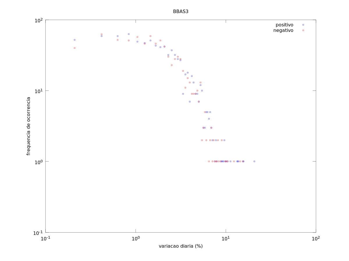
According to Mandelbrot, the variation on commodities and financial assets through time follow a Zipf law. He made a analysis with data from cotton price over a few months. I decided to try it myself and see if it really holds.
I got some financial assets data and observed the frequency of occurrence of variation within certain ranges. The graphics bellow present this result. In the first graphic, the variation (%) range was linearly sliced. In the second graphic, I made a logarithmic spaced slices. The third image has a linearly spaced slices, but the number of slices is quite smaller.
When the number of slices is smaller, we clearly see a straight line, what means a power law holds. When the number of slices is bigger, it behaves like a line with a saturation for very frequent values.
Petrobras


Bovespa index


Banco do Brasil


"But economics is like sand, not like water. Decisions are discrete, like the grains of sand, not continuous, like the level of water. There is friction in real economics, just like in sand. We don't bother to advertise and take our apples to the market when the expected payoff of exchanging a few apples and oranges is too small. We sell and buy stocks only when some threshold price is reached, and remain passive in between, just as the crust of the earth is stable until the force on some asperity exceeds a threshold. We don't continually adjust our holdings to fluctuations in the market. In computer trading, this threshold dynamics has been explicitly programmed into our decision pattern.
Our decisions are sticky This friction prevents equilibrium from being reached, just like the friction of sand prevents the pile from collapsing to the flat state. This totally changes the nature and magnitude of fluctuations in economics.
Economists close their eyes and throw up their hands when it comes to discussing market fluctuations, since there cannot be any large fluctuations in equilibrium theory: "Explanations for why the stock market goes up or down belong on the funny pages," says Claudia Goldin, an economist at Harvard. If this is so, one might wonder, what do economists explain?
The various economic agents follow their own, seemingly random, idiosyncratic behavior. Despite this randomness, simple statistic patterns do exist in the behavior of markers and prices. Already in the 1960s, a few years before his observations of fractal patterns in nature, Benoit Mandelbrot analyzed data for fluctuations of the prices of cotton and steel stocks and other commodities. Mandelbrot plotted a histogram of the monthly variation of cotton prices. He counted how many months the variation would be 0.1% (or
-0.1% ), how many months it would be 1%, how many months it would be 10%, etc. He found a "Levy distribution" for the price fluctuations. The important feature of the Levy distribution is that it has a power law tail for large events, just like the Gutenberg-Richter law for earthquakes. His findings have been largely ignored by economists, probably because they don't have the faintest clue as to what is going on.
Traditionally, economists would disregard the large fluctuations, treating them as "atypical" and thus not belonging in a general theory of economics. Each event received its own historical account and was then removed from the data set. One crash would be assigned to the introduction of program trading, another to excessive borrowing of money to buy stock. Also, they would "detrend" or "cull" the data, removing some long-term increase or decrease in the market. Eventually they would end up with a sample showing only small
fluctuations, but also totally devoid of interest. The large fluctuations were surgically removed from the sample, which amounts to throwing the baby outwith the bathwater. However, the fact that the Iarge events follow the same behavior as the small events indicates that one common mechanism works for all scales -- just as for earthquakes and biology.
How should a generic model of an economy look? Maybe very much like the punctuated equilibrium model for biological evolution described in Chapter 8. A number of agents (consumers, producers, governments, thieves, and economists, among others) interact with each other. Each agent has a limited ser of options available. He exploits his options in an attempt to increase his happiness (or "utility function" as the economists call it to sound more scientific), just as biological species improve their fitness by mutating. This affects other agents in the economy who now adjust their behavior to the new situation. The weakest agents in the economy are weeded out and replaced with other agents. or they modify their strategy, for instance by copying more successful agents.
This general picture has not been developed yet. However, we have constructed a simplified toy model that offers a glimpse of how a truly interactive, holistic theory of economics might work."
(How Nature Works: The Science of Self-Organized Criticality, Per Bak)
segunda-feira, 8 de novembro de 2010
Pseudoscience
"As pointed out by the philosopher Karl Popper, prediction is out best means of distinguishing science from pseudoscience. To predict the statistics of actual phenomena rather than the specific outcome is a quite legitimate and ordinary way of confronting theory with observarions". (How Nature Works: The Science of Self-Organized Criticality, Per Bak)
quinta-feira, 14 de outubro de 2010
search tips

Basic
- "+" - Result must contain word
- "-" - Result must not contain word
- "OR" and "|" - Applied between two words, it will find "this or that", or both. The "OR" operator must be uppercase and have a space between the 2 words on each side. The "|" operator does not need a space between the words
- " "" " - Finds an exact match of the word or phrase
- "~" - Looks for synonyms or similar items. Eg: "~run" will match runner's and marathon
- ".." - Indicates that there's a range between number. Eg: 100..200 or $100..$200
- "*" - Matches a word or more. Eg: "Advanced * Form" finds "Advanced Search Form"
- "word-word" - All forms (spelled, singe word, phrase and hyphenated
Important
- "site:" - Search only one website or domain. Eg: "PC site:wazem.org" will find PC within wazem.org
- "filetype:" or "ext:" - Search for docs in the file type. Eg: "Linux tutorial filetype:pdf" will find Linux tutorial in the pdf format
- "link:" - Find linked pages (pages that point to the URL)
- "define:" - Provides definition for a word or a phrase
- "cache:" - Display Google's cached version of a web page.
- "info:" - Info about a page
- "related:" - Websites related to the URL
- "allinurl:" - All words must be in the URL
- "allintitle:" - All words must be in the title of the page
- "intittle:" - Match words in the title of the page
- "source:" - News articles from a specific source
Calculations
- "+ - * /" - Normal math signs. Eg: 12 * 4 + 2 - 1 /2
- "% of" - Percentage. Eg:10% of 100
- "^" or "**" - Raise to a power
- units "in" units - Convert Units (currency, measurements, weight). Eg: 300 lbs in Kg, 40 in hex
Others
- "book" or "books" - Search books. Eg: book "LPI Linux Certification in a Nutshell"
terça-feira, 24 de agosto de 2010
spoken english statistics
In order to approximate the frequency of occurrence of phones in spoken english, I used the Gutenberg Project database to get written texts and the CMU Pronouncing Dictionary to get a phonetic transcription of those words.
I used the top 100 books on the list of Gutenberg database. With them I cound build a list of 179,044 types and 14,144,013 tokens. Just to state a comparison, "the Second Edition of the 20-volume Oxford English Dictionary contains full entries for 171,476 words in current use, and 47,156 obsolete words. To this may be added around 9,500 derivative words included as subentries"(see the reference). That builds a total of 228,132 entries. So have around 78% of the entries of the Oxford Dictionary.
With this data at hand and some perl scripting, I made the following lists and ordered them by the frequency of occurrence:
1. list of words;
2. list of phones;
3. list of diphones;
4. list of triphones;
5. list of quadriphones;
6. an interface to browse the data (click on the image bellow);

7. log-log graphic of word rank vs. word frequency;

8. log-log graphic of phone rank vs. phone frequency;

Exponential fit of the data:

Semi-logy plot:

9. log-log graphic of diphone rank vs. diphone frequency;

10. log-log graphic of triphone rank vs. triphone frequency;

11. log-log graphic of quadriphone rank vs. quadriphone frequency;

12. frequency of occurrence of a phone given that a certain phone occurred before;

13. frequency of occurrence of a phone given that a certain phone occurs after;

14. Conditiona probability of occurrence of a given phone given that another has occurred.

14. the kullback-leibler distance (relative entropy) between the phones in english and a uniform distributed random variable is: 0.48363 bits;
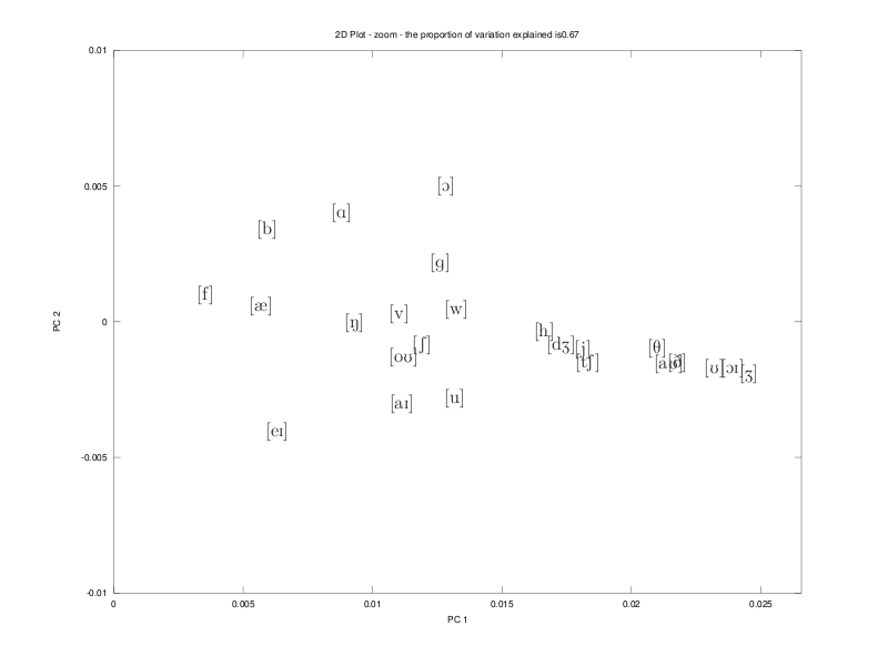
15. considering as a dissimilarity measure between two phones the sum of their individual frequency of occurrence minus the frequency of occurrence of the diphone with this pair of phones, we get the following dissimilarity matrix and we peform a MDS of the data, as shown bellow.


zoom:

16. Words letters-length

17. Frequency of occurrence of words with a certain letters-length normalized by the number of possible permutations of letters with repetition with the same length.

18. Average number of letters in a word across word's rank

19. Words phones-length

20. Frequency of occurrence of words with a certain phonemic-length normalized by the number of possible permutations of phones with repetition with the same length.

21. Average number of phones in a word across word's rank

22. Cumulative probability of phones. The 8 first most frequent phones ([ə, t, n, s, ɪ, r, d, l]) account for half of all phones occurrences in the data.

23. Here are present two types of graphics to verify the contribuition of words frequency to the final phones frequency. The upper plot shows the occurrence of words with a certain phone. The lower one show an extimation of the probability of occurrence of a certain phone across the rank of words.

I used the top 100 books on the list of Gutenberg database. With them I cound build a list of 179,044 types and 14,144,013 tokens. Just to state a comparison, "the Second Edition of the 20-volume Oxford English Dictionary contains full entries for 171,476 words in current use, and 47,156 obsolete words. To this may be added around 9,500 derivative words included as subentries"(see the reference). That builds a total of 228,132 entries. So have around 78% of the entries of the Oxford Dictionary.
With this data at hand and some perl scripting, I made the following lists and ordered them by the frequency of occurrence:
1. list of words;
2. list of phones;
3. list of diphones;
4. list of triphones;
5. list of quadriphones;
6. an interface to browse the data (click on the image bellow);
7. log-log graphic of word rank vs. word frequency;

8. log-log graphic of phone rank vs. phone frequency;

Exponential fit of the data:

Semi-logy plot:

9. log-log graphic of diphone rank vs. diphone frequency;

10. log-log graphic of triphone rank vs. triphone frequency;

11. log-log graphic of quadriphone rank vs. quadriphone frequency;

12. frequency of occurrence of a phone given that a certain phone occurred before;

13. frequency of occurrence of a phone given that a certain phone occurs after;

14. Conditiona probability of occurrence of a given phone given that another has occurred.

14. the kullback-leibler distance (relative entropy) between the phones in english and a uniform distributed random variable is: 0.48363 bits;
15. considering as a dissimilarity measure between two phones the sum of their individual frequency of occurrence minus the frequency of occurrence of the diphone with this pair of phones, we get the following dissimilarity matrix and we peform a MDS of the data, as shown bellow.


zoom:
16. Words letters-length

17. Frequency of occurrence of words with a certain letters-length normalized by the number of possible permutations of letters with repetition with the same length.

18. Average number of letters in a word across word's rank

19. Words phones-length

20. Frequency of occurrence of words with a certain phonemic-length normalized by the number of possible permutations of phones with repetition with the same length.

21. Average number of phones in a word across word's rank

22. Cumulative probability of phones. The 8 first most frequent phones ([ə, t, n, s, ɪ, r, d, l]) account for half of all phones occurrences in the data.

23. Here are present two types of graphics to verify the contribuition of words frequency to the final phones frequency. The upper plot shows the occurrence of words with a certain phone. The lower one show an extimation of the probability of occurrence of a certain phone across the rank of words.

domingo, 22 de agosto de 2010
semantic web
I have just made my first prototype of a semantic web. :)
First I listed the occurences of words placed just by a certain word. The list bellow shows the occurence of words adjacent to the portuguese word 'casa'.
Using this list and the list of the words in this list I built a semantic web!

See other examples:
ainda
depois
ele
quando
tudo
casa
disse
era
tempo
First I listed the occurences of words placed just by a certain word. The list bellow shows the occurence of words adjacent to the portuguese word 'casa'.
era : 41
dono : 35
minha : 35
sua : 30
nossa : 30
estava : 30
verde : 28
foi : 25
porta : 24
dona : 21
velha : 19
me : 18
esta : 18
rua : 18
dele : 18
entrou : 18
ir : 17
dela : 17
chegou : 16
noite : 15
fora : 13
ia : 12
...
Using this list and the list of the words in this list I built a semantic web!
See other examples:
ainda
depois
ele
quando
tudo
casa
disse
era
tempo
terça-feira, 17 de agosto de 2010
word frequency
Here is the process I made to create a frequency list of portuguese words using all the text from Machado de Assis available at http://machado.mec.gov.br/. In the total, this database has 1.645.474 tokens and 62.809 types.
First download all pdfs.
Then convert everything into text.
Then you just need to run my perl script to get the list of words and their occurancy.
Get the script here.
Voilà! And here is the result!
Get the complete list here.

First download all pdfs.
mkdir pdf
cd pdf
wget http://machado.mec.gov.br/arquivos/pdf/romance/marm01.pdf
wget http://machado.mec.gov.br/arquivos/pdf/romance/marm02.pdf
wget http://machado.mec.gov.br/arquivos/pdf/romance/marm03.pdf
...
Then convert everything into text.
for file in $( ls pdf/*.pdf );
do echo $file; outfile=${file//pdf/txt};
pdftotext -enc UTF-8 $file $outfile;
done
Then you just need to run my perl script to get the list of words and their occurancy.
#!/usr/bin/perl
my $dirname = $ARGV[0];
my %count_of;
opendir(DIR, $dirname) or die "can't opendir $dirname: $!";
while (defined($filename = readdir(DIR))) {
   open (FILE, $dirname . $filename);
   while () {
      chomp;
      $_ = lc $_;
      $_ =~ s/\d+/ /g; # remove all numbers
      $_ =~ s/[^a-zA-Z0-9_áéíóúàãõâêôçü]+/ /g;
      #$_ =~ s/\xC3//g; # remove strange one
      foreach my $word ( split /\s+/, $_){
          $count_of{$word}++;
      }
   }
   close (FILE);
}
closedir(DIR);
print "All words and their counts: \n";
foreach $value (sort {$count_of{$b} <=> $count_of{$a} } keys %count_of)
{
  print "$value : $count_of{$value}\n";
}
Get the script here.
Voilà! And here is the result!
All words and their counts:
a : 75485
que : 69366
de : 66929
o : 61165
e : 57056
não : 34354
se : 28067
do : 25059
um : 24125
da : 21992
os : 19764
é : 18307
uma : 16521
em : 15381
com : 14954
as : 14793
para : 13114
mas : 12390
lhe : 11922
me : 10966
ao : 10962
era : 10340
por : 10266
no : 10114
mais : 9148
na : 9003
à : 8719
como : 8506
dos : 7669
eu : 6972
ou : 6696
ele : 6310
foi : 5445
das : 5305
há : 5215
nem : 5169
sem : 4387
quando : 4283
disse : 4140
já : 3924
ela : 3815
ser : 3774
nos : 3687
tudo : 3537
ainda : 3514
só : 3402
depois : 3358
tempo : 3137
casa : 3098
...
Get the complete list here.

domingo, 18 de julho de 2010
Combination
Here is a simple function for Octave/MatLab I wrote to create the combinations of the numbers in a vector. Suppose you want to get the possible combinations of the numbers [1 2 3 4] arrenged in 3, what would give you [1 2 3], [1 2 4], [1 3 4] and [2 3 4]. You just have to use the function bellow calling X = combinations([1 2 3 4],3), and X will be the matrix with all combinations.
function X = combinations(x,k)
%
%  X = combinations(x,k)
%  Create all combinations (without repetition) of the
%  elements in x arragend in groups of k items.
%  example:
%  x=[1 2 3 4];
%  X = combinations(x,3)
%  X =
%     1   2   3
%     1   2   4
%     1   3   4
%     2   3   4
%

if(size(x,1) > size(x,2)), x = x'; end;
n = length(x);
X = [];
if(k == 1),
  X = x';
else
for l = 1 : n-k+1,
    C = nchoosek(n-l,k-1);
    xtemp = x;
    xtemp(1:l) = [];
    X = [X;  [repmat(x(l),C,1) combinations(xtemp,k-1)] ];
end;
end;
quinta-feira, 15 de julho de 2010

quarta-feira, 14 de julho de 2010
Subtitles on PS3
Unfortunately the only way I found, until now, to play downloaded videos with subtitles on my PS3 is using a tool called AVIAddXSubs. This tool create a DivX video by adding a source video (.avi, .mpg. etc) and its subtitle (.srt). The subtitle is added to the DivX container (the DivX Media Format (DMF) has support to multiple subtitles, multiple audio tracks and multiple video streams, among other things, just like Matroska). Although AVIAddXSubs is a Windows program, it might run on Linux, thanks to Wine. I have just tried it and it did work! I could get my video playing on my PS3 with subtitles. :)
quinta-feira, 1 de julho de 2010
models
(...) The value of a model is that often it suggests a simple summary of the data in terms of the major systematic effects together with a summary of the nature and magnitude of the unexplained of random variation. (...)
Thus the problem if looking intelligently at data demands the formulation of patterns that are thought capable of describing succinctly not only the systematic variation in the data under study, but also for describing patterns in similar data that might be collected by another investigator at another time and in another place.
(...) Thus the very simple model
\[ y = \alpha x + \beta ,\]
connecting two quantities y and x via the parameter pair (α,β), defines a straight-line relationship between y and x. (...) Clearly, if we know α and β we can reconstruct the values of y exactly from those if x (...). In practice, of course, we never measure the ys exactly, so that the relationship between y and x is only approximately linear. (...)
The fitting of a simple linear relationship between the ys and the xs requires us to choose from the set of all possible pairs of parameters values a particular pair (a, b) that makes the patterned set $\hat{y}_1,\ldots,\hat{y}_n$ closest to the observed data. In order to make this statement precise we need a measure of 'closeness' or, alternatively, of distance or discrepancy between the observed ys and the fitted $\hat{y}$s. Examples of such discrepancy functions include the $L_1$-norm
\[S_1(y,\hat{y}) = \sum | y_i - \hat{y}_i | \]
and the $L_\infty$-norm
\[S_\infty(y,\hat{y}) = \max_i | y_i - \hat{y}_i | .\]
Classical least squares, however, chooses the more convenient $L_2$-norm or sum of squared deviations
\[S_2(y,\hat{y}) = \sum ( y_i - \hat{y}_i )^2 \]
as the measure of discrepancy. These discrepancy formulae have two implications. First, the straightforward summation of individual deviations, either $| y_i - \hat{y}_i |$ or $( y_i - \hat{y}_i )^2$, each depending on only one observation, implies that the observations are all made on the same physical scale and suggests that the observations are independent, or at least that they are in some sense exchangeable, so justifying an even-handed treatment of the components. Second, the use of arithmetic differences $y_i - \hat{y}_i$ implies that a given deviation carries the same weight irrespective of the value of $\hat{y}$. In statistical terminology, the appropriateness of $L_p$-norms as measures of discrepancy depends on stochastic independence and also on the assumption that the variance of each observation is independent of its mean value. Such assumptions, while common and often reasonable i practive, are by no means universally applicable.
(Generalized Linear Models, P. McCullagh and J.A. Nelder)
sábado, 19 de junho de 2010
Veja desenvolve novo método para testar indenpência de duas variáveis aleatórias.
Na edição de 16 de Junho de 2010, a Veja mostra um novo método para testar indenpência de duas variáveis aleatória, no caso em questão, aplicado para analisar a independência das Eleições e Copa do Mundo.
in reference to: Eleições: Equilíbrio inédito na corrida presidencial - Edição 2169 - Revista VEJA (view on Google Sidewiki)segunda-feira, 14 de junho de 2010
Create your own booklets

Here is a easy way to create your own booklets and print'em... easy and fast.
You just have to put the paper, run the script, and change the paper when asked to.
(*note: there is no need to reorder the pages... the script does it automatically)
Here is a script to do it all:
#!/bin/bash
file=$1
pdf2ps $file /tmp/${file%%.pdf}.ps
psbook /tmp/${file%%.pdf}.ps /tmp/out.ps
psnup -2 /tmp/out.ps /tmp/out2up.ps
ps2pdf /tmp/out2up.ps ${file%%.pdf}-booklet.pdf
echo Do you want to print the booklet now? \(y\)es or \(n\)no:
read PRINT
if [ "$PRINT" = "y" ]; then
   lp -o page-set=odd ${file%%.pdf}-booklet.pdf
   echo change paper now! \(no need to reorder pages\)
   read PRINT
   lp -o page-set=even -o outputorder=reverse ${file%%.pdf}-booklet.pdf
fi
you may download it here.
quarta-feira, 2 de junho de 2010
pdfposter
Go to official pdfposter website here.
This tool is very simple and good. You can split a PDF document into several to create a poster. See the example bellow:
pdfposter -p 4x4a4 /tmp/drawing.pdf /tmp/out.pdf
input: 1 page, A0, pdf file:
drawing.pdf

output: 16 pages, A4, pdf file:
out.pdf

But there is a problem... printers usually have a printable area, so you need to add a margin to your document in order to don't lose anything when you print it. Here is how I did it for the example above.
First, use pdfposter to create a smaller version (160x247mm, that means 2.5mm of top, bottom, left and right margins).
pdfposter -m160x247mm -pA0 drawing.pdf out.pdf
After that, create a TeX document that will include this pdf, place each page inside a A4 page and include cropping marks. Here is the source code:
\documentclass{article}
% Support for PDF inclusion
\usepackage[final]{pdfpages}
% Support for PDF scaling
\usepackage{graphicx}
\usepackage[dvips=false,pdftex=false,vtex=false]{geometry}
\geometry{
   paperwidth=160mm,
   paperheight=247mm,
   margin=2.5mm,
   top=2.5mm,
   bottom=2.5mm,
   left=2.5mm,
   right=2.5mm,
   nohead
}
\usepackage[cam,a4,center,dvips]{crop}
\begin{document}
% Globals: include all pages, don't auto scale
\includepdf[pages=-,pagecommand={\thispagestyle{plain}}]{/tmp/out.pdf}
\end{document}
And... voilà! Here is the final pdf. And it page will be like this:

Assinar:
Postagens (Atom)